

Summary & Key Findings
A little-known concept called Shannon’s Demon may actually be a vital tool for increasing returns and minimizing risks in investor portfolios over time.
As we’ll show, the mathematical underpinnings of Shannon’s Demon can actually make it possible to generate positive returns at the portfolio level, even when all of the portfolio’s individual holdings are expected to produce zero, or even negative, returns over time.
Given the market environment as of this writing, which is characterized by near-zero bond yields and all-time high U.S. stock valuations, we feel the concepts that we outline below and the rebalancing return premiums that can be generated have the potential to offer investors attractive alternative paths to portfolio returns, all while avoiding incremental portfolio risks.
Introduction
There is a fascinating mathematical concept that remains little-known to folks in the investment industry (individuals and professionals alike), despite having the potential to materially enhance investor portfolios over time. This concept is oddly enough referred to as “Shannon’s Demon” – named after the renowned MIT mathematician, Claude Shannon. (Note: we know the “Demon” part seems a bit odd, but rest assured, it is nothing diabolical or demonic in nature. It actually stems from an area of thermodynamics, but we will spare everyone with the boring details there.)
The general idea behind Shannon’s Demon is that two uncorrelated assets, each with zero expected long-term returns, can actually produce a combined portfolio that consistently generates positive returns if intelligently balanced and rebalanced at regular intervals. Sounds too good to be true, we know. But, we will show how this is possible, and it doesn’t require a PhD understanding of number theory or quantum mechanics either.
Furthermore, given today’s investment landscape, which is characterized by near-zero interest rates and diminished long-term return estimates on risk-based assets, we felt it might be a good time to shed some light on Shannon’s Demon and how it might be harnessed to improve portfolio results over time, in spite of the current scarcity of assets with attractive return profiles.
A Simple Walk Through of Shannon’s Demon
Claude Shannon was an American mathematician, MIT professor, electrical engineer, and World War II cryptographer - and is known today as “the father of information theory”.
Ultimately, what he was able to show with his concept of Shannon’s Demon was that you could take a volatile asset that never would earn any long-term return (i.e., it just randomly moved up and down over time), and convert it into a valuable contributor to a wealth generating portfolio through the simple process of rebalancing.
To illustrate this concept, you could consider a simple coin-flip game where you make a 50% return on your money if the coin lands on heads, or lose 33.3% of your money if the coin lands on tails. This simple game has a expected long-term return of zero. For instance, let’s say you start with $100. You then invest it all in the coin flip game, the coin lands on heads (so in this instance you win), and you make a 50% return - resulting in a new portfolio value of $150. On the next flip you invest all $150 in the coin flip game, the coin lands on tails, so you lose 33.3% and are then back at your original $100. If the coin is a fair coin, you should expect to broadly oscillate around your original $100 bankroll without making or losing any money over the long haul. The math behind this is detailed a bit more extensively in Figure 1 and can be better conceptually visualized through the graph in Figure 2 below.
Figure 1: Coin Flip Game without Rebalancing – First 10 Flips Example
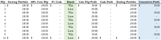
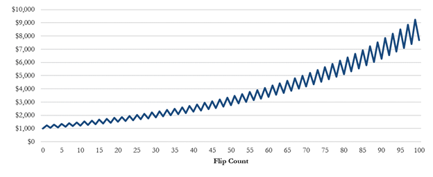
Figure 2: Coin Flip Game without Rebalancing – Example Equity Curve

Now here is where things get pretty interesting. What if you decided to rebalance 50% of your bankroll into cash after each coin-flip, regardless of whether you win or lose? Would that change your long-term return expectations? Intuitively, most people would not think so. The coin-flip game has a zero expected return, and cash has a zero expected return (at least in this example), so how would this change things? Well, it changes things quite a bit, because it converts two zero-expectancy return streams into a wealth generating machine.
To illustrate this, let’s walk through a few of the steps of the coin-flip game with our new rebalancing approach.
Portfolio starts with $100: $50 goes into the coin-flip game and $50 goes into cash.
Coin lands on heads: Win $25 (50% return) on the coin-flip and win $0 on the cash.
Portfolio now has $125, we rebalance: $62.5 into the coin-flip and $62.5 into cash.
Coin lands on tails: Lose $20.83 (33.3% loss) on the coin-flip and lose $0 on the cash.
Portfolio now has $104.17, we rebalance: $52.08 into the coin-flip and $52.08 to cash.
Coin lands on heads: Win $26.04 on the coin-flip and win $0 on the cash.
Portfolio now has $130.21, we rebalance, and so on…
Figures 3 & 4 present this simple example in better detail and the new rebalanced portfolio growth graphically.
Figure 3: Coin Flip Game with 50/50 Rebalancing – First 10 Flips Example

Figure 4: Coin Flip Game with 50/50 Rebalancing – Example Equity Curve
Now you might be wondering, what if the coin doesn’t always evenly switch between heads and tails? What if it truly is a random 50/50 chance for each flip, leading to potential winning and losing streaks like you would expect in real life? Well, we can actually simulate this randomness using a computer.
More specifically, we can tell a computer to randomly choose between heads and tails 1,000 times to simulate 1,000 randomized coin flips. We can then string these coin-flip results together sequentially to determine our simulated profit & loss profile over time. And finally, for robustness’ sake, we can then repeat this simulated process (say 100 times) to really get a good holistic view of what the true expectations from playing the coin-flip game should be on average.
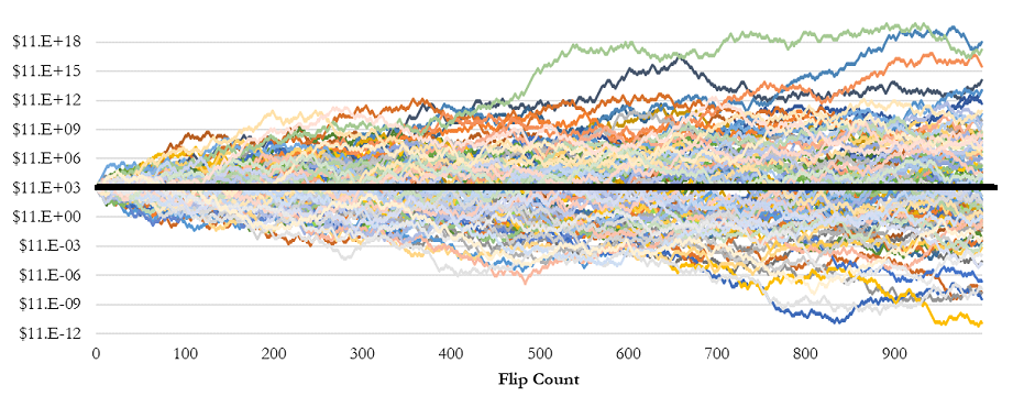
If we first simulate the coin-flip game without rebalancing into cash, we end up with the simulated profit & loss curves presented in Figure 5 below. We can see that there is a fair amount of dispersion (lots of winners and lots of losers), but in aggregate they are all essentially centered around the zero line (i.e. no long-term returns are generated on average) - which is what we would expect, as there is mathematically a zero expected return from playing this game.
Figure 5: Coin Flip Game without Rebalancing – 100 Simulated Equity Curves
Now, what if we took the same 100 simulations, but this time we rebalanced 50% of our bankroll into cash after each simulated coin flip? The new rebalanced results are presented in Figure 6 below.
Figure 6: Coin Flip Game with 50/50 Rebalancing – 100 Simulated Equity Curves

Bingo! As we can see in Figure 6, even with random coin flips, the expectancy of every single simulation is now consistently positive. We have just created a return producing portfolio from two assets that have zero expected returns and zero wealth generation capabilities on their own.
Now, obviously this is just a simple example illustrated by a hypothetical coin-flip game, and it is not likely something in which we would be able to invest our hard-earned money in real life. That being said, the main concepts still very much apply to real world investing and optimizing investment portfolios through time – albeit with a bit more complexity and sophisticated computations to account for changing market dynamics.
So Why Does Shannon’s Demon Work?
The reason why we are able to generate a positive return just by simply rebalancing is because we are effectively reducing a powerful negative force called “volatility drag”.
To better understand volatility drag and the power of it, assume you have $100 to invest. In the first year, you make a 10% return. Then in the second year, you lose 10%. Intuitively, many people would think you’re back to breakeven, but you’re not. You’re actually down 1% from where you started – $99. Moreover, the greater the size of these return swings (i.e. the greater the volatility), the more the volatility drag increases – and it grows exponentially! For instance, if your return swings were 20% instead, then you’d be down 4% after the second year. Even though volatility only doubled (10% to 20%), the volatility drag quadrupled (-1% to -4%).
In the case of Shannon’s Demon and figuring out why we actually make money over time in two zero-return assets, a better way of looking at the problem is through analyzing how volatility drag converts an arithmetic average return into a geometric average return (or compound return).
For instance, our simple coin-flip example above actually has an arithmetic average expected return of roughly 8.4% (e.g. (50% - 33.3%) ÷ 2), but the expected geometric average return (or compound return) over time is still zero – and it is this geometric average return that really matters to us, as this is the actual return in our account and what we ultimately get to take home.
So, what causes the difference between our 8.4% arithmetic average return and the 0% geometric average return? Where does all of that return go? Once again, the volatility drag takes it away! The formula to approximate this relationship is as follows:
*Note: Volatility Drag ≈ Volatility2 ÷ 2
Coin-Flip Game: 8.4% - (42%2 ÷ 2) ≈ 0% (Approximately)
As noted above, the volatility drag grows exponentially as volatility increases. So, when we rebalance and reduce overall portfolio volatility through diversification, we have the opportunity to reduce the volatility drag by a greater degree than the amount we reduce our expected arithmetic average return. This can then enable us to convert an expected 0% geometric return into a positive geometric return by simply reducing volatility through rebalancing into uncorrelated or anti-correlated assets.
More specifically, by rebalancing 50% into cash before each flip, two important things happen. First, you decrease your arithmetic average return expectations by 50% (remember the arithmetic average is not important to us, only the geometric return is). Secondly, and more importantly, you reduce volatility drag, and by a much larger degree – in this case by a whopping 75%! When these dynamics are applied to our coin flip example above, we end up converting our original 0% expected geometric return to a 2% expected geometric return – and all we had to do was rebalance.
In summary, you end up making more return over time by strategically losing less to volatility drag. This is one of the many benefits of diversification and why it’s often referred to as “the only free lunch in investing.”
Why Do We Care?
We at RQA are focused on investing as intelligently as possible (selfishly and for our clients), and the concepts of Shannon’s Demon and volatility drag have tremendous implications in the world of investments and portfolio management – particularly today, as bond yields remain at historic lows and expected long-term returns on many other asset classes are estimated to be fairly muted given current lofty valuation levels.
As we’ve illustrated above, it is possible to generate incremental returns just by reducing volatility drag within the portfolio, and this can be done by simply rebalancing across uncorrelated assets – even those that are expected to produce little-to-no return on their own. (As a reminder, both cash and the coin flip game had zero return expectations on their own, but when combined and rebalanced they produced something meaningfully positive.)
Given these concepts, the exciting part to us is that we don’t necessarily need to be confined to the near-zero yields and low expected returns in individual asset classes today. By combining a truly diverse set of assets and rebalancing regularly based on how they zig and zag around one another, we know it is possible to generate portfolio returns that exceed the expected average of the individual component holdings, all while reducing risk at the same time.
Some Final Thoughts
Interest rates have remained near the zero-bound for over a decade now, and investors are still on an exhaustive hunt for any kind of meaningful yield in their portfolios – and we are often seeing folks throw reason and sound investing principles out the window in trying to find it.
The inherent dilemma here is that anything these days offering a high yield in any traditional form, whether through dividends or interest, are often too good to be true in some way. Typically, either the risks of material loss on principal in these “high-yield” investments are either very high (i.e. low credit quality or options-related blow-up risk), or they are effectively paying you a “yield” by returning your own money back to you – so not really a yield at all, even though it might feel like it (i.e. annuities or some of the newly branded high-yield ETFs).
As we’ve highlighted above, the good news is that you don’t necessarily need to find some elusive investment opportunity with a high dividend or interest rate to produce attractive yields from your portfolio. In fact, you can use the mathematical concepts behind Shannon’s Demon to produce returns from assets that aren’t even expected to produce positive returns at all (though finding assets with positive expected returns is certainly more advantageous), all while simultaneously reducing portfolio risk.
In today’s market, we find that when investors choose to intelligently deploy these concepts across a portfolio of lowly correlated assets (even those without any inherent yield), we can start to see incremental returns or rebalancing premiums shine through, all while meaningfully reducing portfolio risk and improving return consistency over time.
To receive RQA Research and Updates, sign up with your email.
Disclaimer: These materials have been prepared solely for informational purposes and do not constitute a recommendation to make or dispose of any investment or engage in any particular investment strategy. These materials include general information and have not been tailored for any specific recipient or recipients. Information or data shown or used in these materials were obtained from sources believed to be reliable, but accuracy is not guaranteed. Furthermore, past results are not necessarily indicative of future results. The analyses presented are based on simulated or hypothetical performance that has certain inherent limitations. Simulated or hypothetical trading programs in general are also subject to the fact that they are designed with the benefit of hindsight.